Also available in Italian: La tesi in italiano.
Streaming platforms hold tens of millions of tracks. To organize them, recommend new ones or read listening histories, they need to group songs by how they sound. Genre tags are not reliable enough for that, because different people tag the same song differently.
Grouping songs by sound became my bachelor’s thesis in Computer Engineering at the University of Modena and Reggio Emilia (UNIMORE), Department of Engineering “Enzo Ferrari” (academic year 2024/25, advisor Prof. Francesco Guerra, defended October 8, 2025): can unsupervised clustering algorithms discover musically meaningful structure from raw audio features alone? I compared three algorithms from three different families (K-Means, DBSCAN, and Spectral Clustering) on two datasets, judging them with internal metrics and a post-hoc genre analysis. The full pipeline is open source on GitHub(opens in a new tab).
Why clustering without labels
Clustering groups data points by similarity without ever seeing a label during training. This matters for music, because genre tags are noisy, subjective and incomplete. Is a track “rock” or “metal”? “Techno” or “trap”? Human curators disagree, artists blend styles, and many songs are hybrids. A model trained on those labels learns the same disagreements.
The unsupervised approach starts from the data. Each track becomes a vector of acoustic measurements, similar vectors are grouped, and only afterwards do we check whether the groups line up with genres. Genres are used to check the result, never to train. If clusters emerge that collect, say, nearly all classical pieces together without ever being told what “classical” is, the features capture something real about the sound.
Two datasets, 167 features per track
I worked with two complementary datasets:
- GTZAN, the standard benchmark for music genre classification, introduced by Tzanetakis and Cook. It has 1000 tracks of 30 seconds each, 100 for each of 10 genres: blues, classical, country, disco, hip-hop, jazz, metal, pop, reggae and rock.
- Custom dataset: 684 tracks from my own Spotify playlists, labeled with 5 deliberately distinct macro-genres: techno (208), classical (187), rock & metal (157), funk (69), trap (63). These are my playlists, so the set is biased, and the thesis says so. I chose labels that differ clearly even to a casual listener, so when an algorithm mixes them up, the failure tells us something.
Every track was converted into 167 numerical features with librosa(opens in a new tab): 40 MFCC coefficients (how humans perceive timbre), 72 chroma features across STFT/CQT/CENS variants (harmonic content), spectral descriptors (centroid, bandwidth, rolloff, contrast, flatness), polynomial shape features, tempo and onset statistics, Tonnetz (harmonic atmosphere), zero-crossing rate, RMS energy, and harmonic-percussive separation ratios.
Before any clustering, a strict preprocessing pipeline ran in fixed order: duplicate removal, z-score standardization (mandatory, since Euclidean distances are dominated by the largest-scale features otherwise), and PCA retaining 98% of the variance to fight the curse of dimensionality, where distances in high-dimensional spaces concentrate and stop being discriminative.
A reproducible protocol
All experiments ran through a single Python pipeline built on scikit-learn(opens in a new tab) It runs on the CPU only, and every random component gets a fixed seed, so runs are comparable. For each algorithm I tested a grid of hyperparameters on both datasets:
| Algorithm | Custom grid | GTZAN grid |
|---|---|---|
| K-Means | ||
| Spectral | , | , |
| DBSCAN | , | , |
Each configuration was scored with two internal metrics pulling in opposite directions:
- Silhouette score (higher is better): how much closer each point is to its own cluster than to the nearest neighboring cluster.
- Davies–Bouldin index (lower is better): the average similarity of each cluster with its most similar neighbor, balancing intra-cluster scatter against inter-cluster distance.
The best model per algorithm maximized Silhouette, broke ties with Davies–Bouldin, and had to survive a qualitative check: a PCA projection down to 2 components plus a cluster-by- cluster genre breakdown. Genre data never entered training. It only appeared in these post-hoc reports.
K-Means: the baseline
K-Means partitions points into groups by minimizing the within-cluster variance around centroids:
It assumes compact, roughly spherical clusters and needs upfront. But it is fast, interpretable (each centroid reads as a “typical sound profile” of its group), and a mandatory reference point.
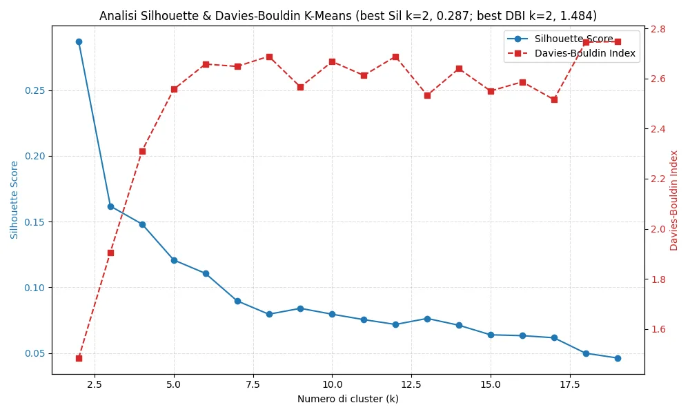
On the custom dataset with , K-Means reached a Silhouette of 0.121 and a Davies–Bouldin of 2.558. The standout result: 98.4% of all classical tracks landed in a single cluster (184 of 190 points, 96.8% pure). Techno and trap largely separated too, while funk collapsed into the rock & metal cluster, with 56 funk tracks sitting next to 122 rock & metal ones, which makes sense: the two share a lot of timbre (driven guitars, similar energy bands).
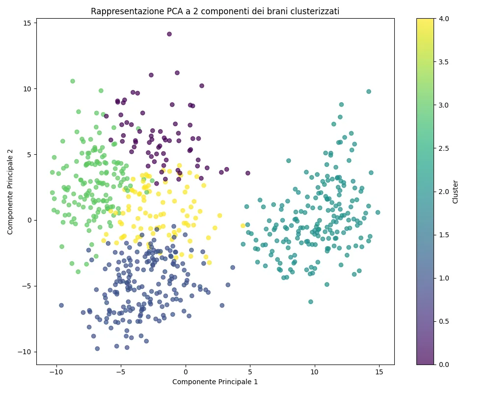
On GTZAN with , scores dropped (Silhouette 0.0635, Davies–Bouldin 2.622), as expected with ten finer-grained genres. Still, 84.9% of metal tracks stayed together, and every cluster was dominated by 1–3 related genres rather than random mixtures: reggae with blues, classical with jazz, pop with hip-hop. The algorithm did not recover genres. It recovered families of similar genres, which matches how the music sounds.
Spectral Clustering: the best scores
Spectral Clustering builds a similarity graph over the data (here with an RBF kernel ), embeds points using the smallest eigenvectors of the graph Laplacian, and runs K-Means in that embedding. It can capture non-convex, curved separations that defeat centroid methods, at the price of delicate graph tuning and higher compute cost.
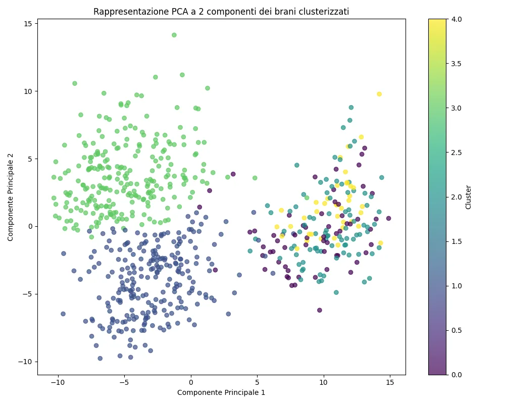
On the custom dataset (, ) it posted the best internal scores of the whole study: Silhouette 0.140, Davies–Bouldin 2.168. 95.7% of funk concentrated in one cluster (alongside rock & metal, that pairing again), techno and trap merged into another, and classical split cleanly from everything else.
On GTZAN (, ): Silhouette 0.0715, Davies–Bouldin 2.484, with 87.1% of metal cohesive. No pure single-genre clusters emerged, but related genres consistently traveled together.
DBSCAN: it did not work
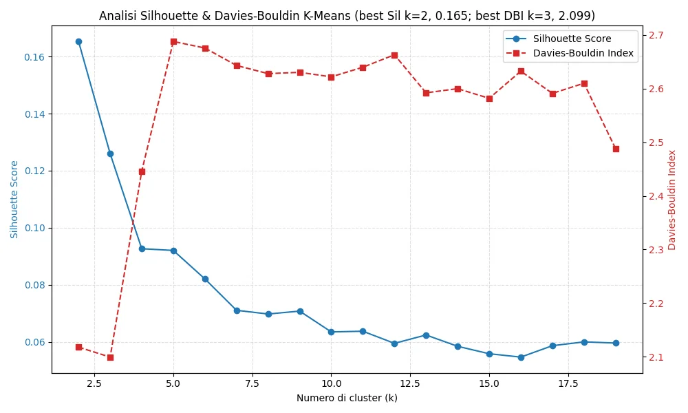
DBSCAN finds dense regions separated by sparse ones, needs no , tolerates arbitrary shapes, and explicitly labels outliers as noise. On paper it looked promising for music. In practice it failed on both datasets: configurations converged to just 1–2 clusters while flagging ~41% of tracks as noise. On the custom dataset the “best” run isolated part of the classical music and dumped nearly everything else into a single mega-cluster plus the noise bin.
The analysis found three causes that add up:
- No separate dense regions: even after PCA, the k-distance plot showed no clear elbow, so no global was principled. Small values labeled everything noise, large values fused everything into one blob.
- Variable density: heterogeneous acoustic features mean some genre regions are dense and others sparse; a single global cannot serve both.
- Continuous stylistic space: hybrid tracks form bridges between genre regions instead of empty gaps, and DBSCAN reads bridges as noise.
Internal metrics computed only on the non-noise points even looked good. They ignore 41% of the data, so they are misleading. A natural next step would be HDBSCAN, which handles variable density hierarchically.
Takeaways
Silhouette values stayed low everywhere (0.06 to 0.14), because songs overlap a lot in feature space. The comparison between algorithms and the genre check afterwards still point the same way:
- Start with K-Means. It is fast and stable, and its clusters are easy to read.
- Spectral Clustering is worth the extra cost when the groups are not linearly separable. It had the best scores and the groupings that made the most sense musically.
- DBSCAN is the wrong tool for dense, high-dimensional, variable-density audio features. Reserve it for data with well-separated density islands.
- Clusters are genre families, not genres: no method recovered ten clean genre bins, because songs themselves are not ten clean bins. Hybrid tracks distribute across clusters, which says as much about genre labels as about the algorithms.
The thesis lists its limits: small datasets, personal bias in the custom set, and qualitative genre labels. Within those limits, unsupervised clustering found real musical structure from the sound alone. Classical and metal ended up in their own clusters almost every time.
The pipeline, the grid searches and the report generators are open source on GitHub(opens in a new tab). Thanks to Prof. Francesco Guerra for advising the thesis (and grazie). Read the Italian version if you prefer.